Importing and Exporting Files

Author

Affiliation

Pennsylvania State University

Published

July 1, 2024

Overview

Until recently, Julia didn’t have a single package to import the majority of file types. However, with the increasing development efforts put into the {Tidier.jl} meta-packages, aimed at recreating the wildly popular set of {tidyverse} R packages in Julia, a new, convenient, single interface exists to the many excellent Julia I/O (input/output) packages. Here, we will explore some common workflows that can utilize the {TidierFiles.jl} package, though more details can be found in the documentation.

File Paths

If you’ve set up your project using {DrWatson}, you should have a number of useful helper functions for you to use in your project (after loading and activating the project with using DrWatson; quickactivate(Project)). Because you created a new folder for the project, Julia will create a Project.toml and a Manifest.toml file in your project folder. This does all the hard work of setting up relative paths, and making sure each project has it’s own list of packages and versions, avoiding any conflicts that may arise when you set up another project with similar packages. To make use of your code and project-specific packages, you simply need to activate the project using {DrWatson}’s quickactivate("Project") function (or with ]activate . if you are in the correct directory).

A relative filepath is simply the steps that need to be taken to find your target file from the current location, e.g., the active file. For example, you may have the following files in a project:

│projectdir
│
├── data
│   └── exp_raw.csv
├── out
│   └── exp_clean.parquet
.
.
.
├── scripts
│   ├── cleaning.jl
│   └── intro.jl
.
.
.
├── Manifest.toml
└── Project.toml

The relative filepath of the exp_raw.csv data file from the intro.jl scripts file is ../data/exp_raw.csv. Here, ../ means look in the parent directory i.e., one directory up from the current location, with the rest pointing to the data/ directory and appropriate file. If you wanted to cleaning.jl file from intro.jl, the relative path would just be cleaning.jl (or alternatively ./cleaning.jl, where ./ means look in the current directory).

Note

Generally you won’t need to refer to other script/ files as they shouldn’t contain functions that are used for calculations, only the scripts that utilize the functions defined in the src/ directory to produce your results. As we’ll come to later, Julia has been designed to make creating and working with packages very simple, which we will take full advantage to minimize the risk of files relying on each other in a circular fashion.

As mentioned, {DrWatson} provides convenience functions to simplify the process of locating files with relative paths. To load a file from the data/ folder, we need to include() it. This effectively finds the file and runs it, so everything defined in it is now available for use. In practice, we can simply use the command include(DrWatson.datadir("filename.jl")) (or drop the DrWatson. package namespace if you brought {DrWatson} into the Main namespace with the using command - see here for more information about namespaces). This helpful function means that the file filename.jl can be loaded from within any file in your project without needing to use multiple ../ calls in the relative path, or specify the absolute filepath. It also means that you can send your code to the REPL and it will execute correctly, which is not a given as the directory that the REPL is started in is usually the project directory, and your current file may be in a subdirectory, so the relative paths to the file to load will be different.

Note

In case you’re wondering what {DrWatson} is doing when it sets up these helper scripts, we can just have a look at the source code. The beauty of Julia is that its speed and expressiveness means that most Julia packages are written in pure Julia and don’t need to resort to lower-level languages for the internals!

Looking at these lines in the source code, we can see that the projectdir() function is effectively a wrapper around the below code, with a check to make sure you have activated the project.

dirname(Base.active_project())

Tip

Because we created the out/ directory to save our processed data files to, it would be useful to have a similar helper function to {DrWatson}’s. We can do that very easily using the following function definition:

outdir(args...) = DrWatson.projectdir("outdir", args...)

Incidentally, this is exactly how {DrWatson} defines it’s helper functions, and states that the functions can take any number of arguments and should join the directory path of the outdir/ and the function arguments. For example, outdir("simulation-files") becomes path-to-project/outdir/simulation-files/.

`{TidierFiles}` Overview

At the time of writing this section, the following file formats can be read and written to using {TidierFiles}:

Delimited files
- .csv read_csv() and write_csv()
- .tsv read_tsv() and write_tsv()/write_table()
- .txt read_delim()
Excel files read_xlsx() and write_xlsx()
- .xlsx
SPSS files read_sav() and write_sav()
- .sav
- .por
SAS files read_sas() and write_sas()
- .sas7bdat
- .xpt
Stata files read_dta() and write_dta()
- .dta
Arrow files read_arrow() and write_arrow()
- .arrow
Parquet files read_parquet() and write_parquet()
- .parquet

Reading and writing files is greatly simplified by using a common interface. To read a file, the general command is read_{format}(path-to-file.{format}) e.g., to read the exp_raw.csv file we would use the command read_csv(DrWatson.datadir("exp_raw.csv")), and to read the exp_clean.parquet file we would use the command read_parquet(outdir("exp_raw.parquet")). If you wish to use the values from the file, rather than just viewing them, you should assign them to a variable e.g. raw_df = read_csv(DrWatson.datadir("exp_raw.csv")).

Writing data to files is similarly simple, just replacing the read_ with write_, and passing in a DataFrame as the first argument. For example, to write a dataframe to a csv file, you simply use the command write_csv(raw_df, outdir("exp_clean.csv")). Currently, all write functions require the use of a DataFrame object, and all read functions return a DataFrame object.

Importing Files

CSV Files from Internet URLs

With {TidierFiles} we can read data from URLs that are hosted on the web. To do this, we can use the read_csv() function and pass in the URL as the first argument, instead of a relative filepath. If the CSV or txt file is hosted on GitHub, you can navigate to the file in GitHub, open up the raw version, and pass the URL to the read_csv()/read_delim() function.

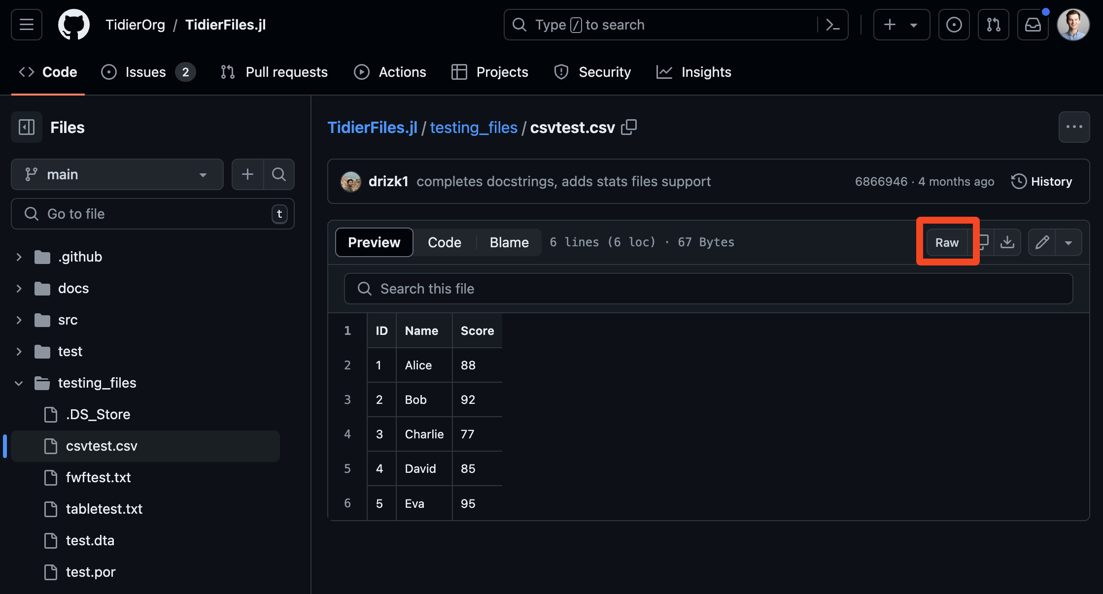
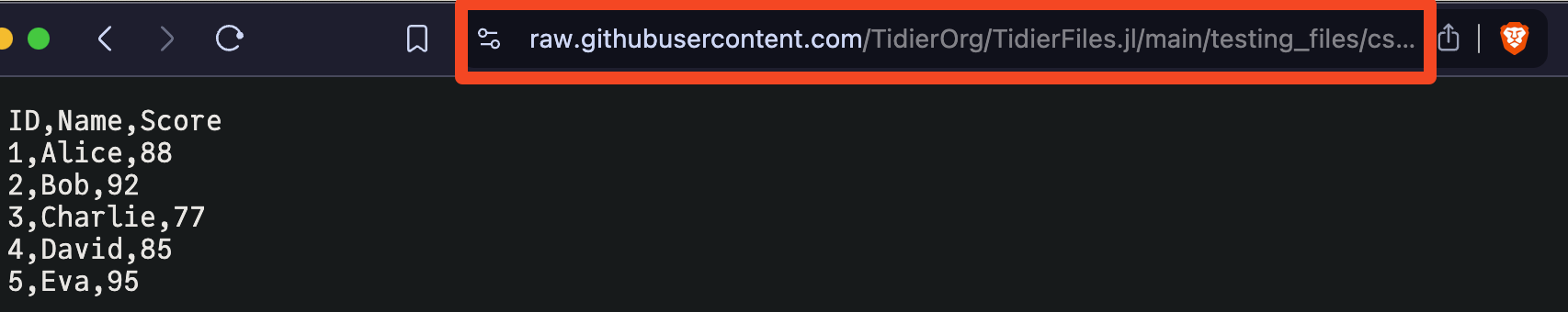
using TidierFiles

read_csv(
    "https://raw.githubusercontent.com/TidierOrg/TidierFiles.jl/main/testing_files/csvtest.csv";
    skip = 1, # skip the first data row
    n_max = 4, # only read the first 4 rows
    col_select = ["ID", "Score"], # only read the "ID" and "Score" columns
    missingstring = ["4"] # replace the value "4" with a missing value representation
)

4×2 DataFrame

Row	ID	Score
	Int64?	Int64
1	2	92
2	3	77
3	missing	85
4	5	95

Specific Excel Sheets & Ranges

While it’s generally preferable to try and use non-proprietary data files that can be read by multiple software tools, such as .csv files, we are sometimes just provided with Excel files (or need to create them). In these situations, we can use {TidierFiles}‘s Excel functions’ to access data from specific sheets, or use the underlying {XLSX} package to read and write Excel files.

To read data from a sheet, we use the sheet = keyword argument of read_xlsx(path-to-file.xlsx, sheet = "sheet-name") function.

Often, Excel sheets contain multiple tables, which may be related to one-another, but should be considered as their own separate entities. In these situations we can use the range = keyword argument of the read_xlsx() function to only read a portion of the Excel sheet.

Missing Data

For delimited and Excel files, it is possible to specify how missing data should be handled on file reads. This is done using the missingstring = keyword argument of the read_{format}() functions, and defaults to "".

Skipping Rows

Your input data files may include a number of header rows that you do not want to include in the resulting dataframes, for example, a data dictionary that lists how values in the main table are coded. These rows can be skipped using the skip = keyword argument of all the read_{format}() functions.

Automated Programming Interfaces (APIs)

Sometimes an API is used to request and access data. Although it sounds very technical and complicated, an API is simply a (documented) method of interacting with a code and data source. In fact, we’ve already been using APIs throughout this book - every package provides a number of functions that are exported and available to end-users, which constitutes an API! Now that we’re a little more comfortable with the notion of an API, let’s see how it is often used in programming: to access data and information from websites.

For this example, we are going to use the Delphi COVIDcast API to collect COVID-19 death incidence data for the USA between 2020 and 2022. Since the beginning of the COVID-19 pandemic, the CMU Delphi team has been collating data from multiple sources and have provided an API for use by researchers and the public alike. As part of this project they have created and R package and a Python package to make interacting with the API easier. While there is not an equivalent Julia package, we can use the API documentation to assist us in downloading the data.

Examining the instructions, we can see we need to use the following base URL: https://api.delphi.cmu.edu/epidata/covidcast/, and that there are a number of required query parameters. To see how we can piece together a query, the Delphi team have provided a number of examples we can use, along with our recently gained understanding of the API requirements. Looking at the examples we can see that each API query starts with ? and uses & to join the query parameters. To fill out the rest of the details, we will look at the example provided in the R package vignette, as this is what we are trying to recreate.

base_url = "https://api.delphi.cmu.edu/epidata/covidcast/?"
data_source = "jhu-csse"
signal = "deaths_incidence_num"
geo = "nation"
geo_values = "us"
time_type = "day"
time_values = "20200415-20221231"

url = base_url * "data_source=" * data_source *
    "&signal=" * signal *
    "&time_type=" * time_type *
    "&geo_type=" * geo *
    "&time_values=" * time_values *
    "&geo_values=" * geo_values

"https://api.delphi.cmu.edu/epidata/covidcast/?data_source=jhu-csse&signal=deaths_incidence_num&time_type=day&geo_type=nation&time_values=20200415-20221231&geo_values=us"

Note

We use the * character to perform string concatenation i.e., to join two or more strings together.

Now that we have our API query, we need to make the request. API calls often use the HTTP internet protocol (the same one that you will be using to access this book), that utilize four verb: GET, SET, PUT, and POST, though we will just focus on GET. In Julia, the {HTTP} package is useful for making HTTP requests, in this case making use of the get() function. Examining the resulting response object, we can see there are a number of properties that can be accessed, but the ones we are interested in are the status and body. The status property provides us with the HTTP status code of the response, i.e., whether the request was successful or not. The body property provides us with the response body, which in this case is the actual data we are interested in.

using HTTP

response = HTTP.get(url)

HTTP.Messages.Response:
"""
HTTP/1.1 200 OK
Date: Wed, 03 Jul 2024 22:24:02 GMT
Content-Type: application/json
Transfer-Encoding: chunked
Connection: keep-alive
Set-Cookie: ******
Set-Cookie: ******
Server: openresty/1.21.4.1
vary: Accept-Encoding
x-my-limit: 60
x-my-remaining: 49
x-my-reset: 1720047589
retry-after: 2146
access-control-allow-origin: *
access-control-allow-methods: GET, POST, OPTIONS
access-control-allow-headers: DNT,User-Agent,X-Requested-With,If-Modified-Since,Cache-Control,Content-Type,Range
access-control-expose-headers: Content-Length,Content-Range
content-encoding: gzip
Strict-Transport-Security: max-age=63072000

{ "epidata": [{"geo_value":"us","signal":"deaths_incidence_num","source":"jhu-csse","geo_type":"nation","time_type":"day","time_value":20200415,"direction":null,"issue":20230303,"lag":1052,"missing_value":0,"missing_stderr":5,"missing_sample_size":5,"value":2596.0,"stderr":null,"sample_size":null},{"geo_value":"us","signal":"deaths_incidence_num","source":"jhu-csse","geo_type":"nation","time_type":"day","time_value":20200416,"direction":null,"issue":20230303,"lag":1051,"missing_value":0,"missing_stderr":5,"missing_sample_size":5,"value":2195.0,"stderr":null,"sample_size":null},{"geo_value":"us","signal":"deaths_incidence_num","source":"jhu-csse","geo_type":"nation","time_type":"day","time_value":20200417,"direction":null,"issue":20230303,"lag":1050,"missing_value":0,"missing_stderr":5,"missing_sample_size":5,"value":2101.0,"stderr":null,"sample_size":null},{"geo_value":"us","signal":"deaths_incidence_num","source":"jhu-csse","geo_type":"nation","time_type":"day","time_value":20200418,"
⋮
280769-byte body
"""

Tip

Although it is good to know how to use string concatenation to create the API query, we can use the query keyword argument to pass a Dictionary of API parameters to the get() function, as shown in the documentation, which is a little cleaner and less prone to errors.

response = HTTP.get(
    base_url;
    query = Dict(
        "data_source" => "jhu-csse",
        "signal" => "deaths_incidence_num",
        "geo" => "nation",
        "geo_values" => "us",
        "time_type" => "day",
        "time_values" => "20200415-20221231",
    )
)

Warning

In practice, you would want to check the status code of the response to make sure that the request was successful, and if not, return an error to stop errors from being propagated throughout your code. In this case, we can just check the response code in the REPL using the following code which asserts that the status code is 200, which is commonly used to denote a successful API request. If the status code is 200, nothing will be printed, and if not, an error will be thrown. An example of an unsuccessful API request would be a 404 error, commonly used to denote that the requested resource does not exist (think about when you came across a 404 error when browsing the internet). HTTP status codes are not hard rules, but they are a standard that most people agree to follow. See here for a full list of HTTP status codes.

@assert 200 == response.status

See this later discussion of Result types for more information on returning errors as values for a better way to handle possible (likely) sources of errors in your code.

first(response.body, 10)

10-element Vector{UInt8}:
 0x7b
 0x20
 0x22
 0x65
 0x70
 0x69
 0x64
 0x61
 0x74
 0x61

Unfortunately the body property is a Vector{UInt8} and we can’t use it in our code, so we need to convert it to a String first before we can manipulate it for plotting purposes.

body = String(response.body)

"{ \"epidata\": [{\"geo_value\":\"us\",\"signal\":\"deaths_incidence_num\",\"source\":\"jhu-csse\",\"geo_type\":\"nation\",\"time_type\":\"day\",\"time_value\":20200415,\"direction\":null,\"issue\":20230303,\"lag\":1052,\"missing_value\":0,\"missing_stderr\":5,\"missing_sample_size\":5,\"value\":2596.0,\"std" ⋯ 280231 bytes ⋯ ",\"source\":\"jhu-csse\",\"geo_type\":\"nation\",\"time_type\":\"day\",\"time_value\":20221231,\"direction\":null,\"issue\":20230224,\"lag\":55,\"missing_value\":0,\"missing_stderr\":5,\"missing_sample_size\":5,\"value\":26.0,\"stderr\":null,\"sample_size\":null}], \"result\": 1, \"message\": \"success\" }"

Note

Once we convert the body to a String, the original data is deleted, so it cannot be used again. To confirm this, we can try calling it again.

response.body

UInt8[]

This is not normally an issue, but it’s something to be aware of. If you really wanted to make sure it was retained, you should instead use the command

body = String(copy(response.body))

Once we have downloaded the JSON data, we need to turn it into something that we can work with in Julia (i.e., a native data structure like a Dictionary). There are a few different options, but here we will use the {Serde.jl} package as it can convert many more file formats, not just JSON. {Serde.jl} is loosely based on the popular {serde.rs} rust library (in that it aims to achieve the same goals), standing for serializing and deserializing data (i.e. converting language specific objects into common formats and back). The function we are interested in here is Serde.parse_json(), which takes the JSON object and converts it into a Dictionary.

Note

JSON is a commonly used data format used to transfer data between web applications and APIs, as well as between many different programming languages. It is non-tabular and hierarchical, and looks a little like a Dictionary entry.

An example from the Delphi COVIDcast API documentation, which states that it returns a JSON object by default, is shown below:

{
  "result": 1,
  "epidata": [
    {
      "geo_value": "06001",
      "time_value": 20200407,
      "direction": null,
      "value": 1.1293550689064,
      "stderr": 0.53185454111042,
      "sample_size": 281.0245
    },
    ...
  ],
  "message": "success"
}

using Serde

parsed = Serde.parse_json(body)

Dict{String, Any} with 3 entries:
  "epidata" => Any[Dict{String, Any}("issue"=>20230303, "geo_type"=>"nation", "…
  "message" => "success"
  "result"  => 1

We can see that {Serde.jl} has converted the JSON into a Dictionary, and the data we are interested in is in the epidata property, which is itself a Vector{Dict{String, Any}} (a vector of dictionaries that has strings for keys and any type for the values).

epidata = parsed["epidata"]

991-element Vector{Any}:
 Dict{String, Any}("issue" => 20230303, "geo_type" => "nation", "lag" => 1052, "sample_size" => nothing, "missing_sample_size" => 5, "value" => 2596.0, "missing_stderr" => 5, "time_value" => 20200415, "geo_value" => "us", "signal" => "deaths_incidence_num"…)
 Dict{String, Any}("issue" => 20230303, "geo_type" => "nation", "lag" => 1051, "sample_size" => nothing, "missing_sample_size" => 5, "value" => 2195.0, "missing_stderr" => 5, "time_value" => 20200416, "geo_value" => "us", "signal" => "deaths_incidence_num"…)
 Dict{String, Any}("issue" => 20230303, "geo_type" => "nation", "lag" => 1050, "sample_size" => nothing, "missing_sample_size" => 5, "value" => 2101.0, "missing_stderr" => 5, "time_value" => 20200417, "geo_value" => "us", "signal" => "deaths_incidence_num"…)
 Dict{String, Any}("issue" => 20230303, "geo_type" => "nation", "lag" => 1049, "sample_size" => nothing, "missing_sample_size" => 5, "value" => 1936.0, "missing_stderr" => 5, "time_value" => 20200418, "geo_value" => "us", "signal" => "deaths_incidence_num"…)
 Dict{String, Any}("issue" => 20230303, "geo_type" => "nation", "lag" => 1048, "sample_size" => nothing, "missing_sample_size" => 5, "value" => 1989.0, "missing_stderr" => 5, "time_value" => 20200419, "geo_value" => "us", "signal" => "deaths_incidence_num"…)
 Dict{String, Any}("issue" => 20230303, "geo_type" => "nation", "lag" => 1047, "sample_size" => nothing, "missing_sample_size" => 5, "value" => 2256.0, "missing_stderr" => 5, "time_value" => 20200420, "geo_value" => "us", "signal" => "deaths_incidence_num"…)
 Dict{String, Any}("issue" => 20230303, "geo_type" => "nation", "lag" => 1046, "sample_size" => nothing, "missing_sample_size" => 5, "value" => 2476.0, "missing_stderr" => 5, "time_value" => 20200421, "geo_value" => "us", "signal" => "deaths_incidence_num"…)
 Dict{String, Any}("issue" => 20230309, "geo_type" => "nation", "lag" => 1051, "sample_size" => nothing, "missing_sample_size" => 5, "value" => 2461.0, "missing_stderr" => 5, "time_value" => 20200422, "geo_value" => "us", "signal" => "deaths_incidence_num"…)
 Dict{String, Any}("issue" => 20230303, "geo_type" => "nation", "lag" => 1044, "sample_size" => nothing, "missing_sample_size" => 5, "value" => 2421.0, "missing_stderr" => 5, "time_value" => 20200423, "geo_value" => "us", "signal" => "deaths_incidence_num"…)
 Dict{String, Any}("issue" => 20230309, "geo_type" => "nation", "lag" => 1049, "sample_size" => nothing, "missing_sample_size" => 5, "value" => 2063.0, "missing_stderr" => 5, "time_value" => 20200424, "geo_value" => "us", "signal" => "deaths_incidence_num"…)
 ⋮
 Dict{String, Any}("issue" => 20230202, "geo_type" => "nation", "lag" => 41, "sample_size" => nothing, "missing_sample_size" => 5, "value" => 207.0, "missing_stderr" => 5, "time_value" => 20221223, "geo_value" => "us", "signal" => "deaths_incidence_num"…)
 Dict{String, Any}("issue" => 20230210, "geo_type" => "nation", "lag" => 48, "sample_size" => nothing, "missing_sample_size" => 5, "value" => 22.0, "missing_stderr" => 5, "time_value" => 20221224, "geo_value" => "us", "signal" => "deaths_incidence_num"…)
 Dict{String, Any}("issue" => 20230224, "geo_type" => "nation", "lag" => 61, "sample_size" => nothing, "missing_sample_size" => 5, "value" => 15.0, "missing_stderr" => 5, "time_value" => 20221225, "geo_value" => "us", "signal" => "deaths_incidence_num"…)
 Dict{String, Any}("issue" => 20230217, "geo_type" => "nation", "lag" => 53, "sample_size" => nothing, "missing_sample_size" => 5, "value" => 29.0, "missing_stderr" => 5, "time_value" => 20221226, "geo_value" => "us", "signal" => "deaths_incidence_num"…)
 Dict{String, Any}("issue" => 20230224, "geo_type" => "nation", "lag" => 59, "sample_size" => nothing, "missing_sample_size" => 5, "value" => 356.0, "missing_stderr" => 5, "time_value" => 20221227, "geo_value" => "us", "signal" => "deaths_incidence_num"…)
 Dict{String, Any}("issue" => 20230224, "geo_type" => "nation", "lag" => 58, "sample_size" => nothing, "missing_sample_size" => 5, "value" => 990.0, "missing_stderr" => 5, "time_value" => 20221228, "geo_value" => "us", "signal" => "deaths_incidence_num"…)
 Dict{String, Any}("issue" => 20230210, "geo_type" => "nation", "lag" => 43, "sample_size" => nothing, "missing_sample_size" => 5, "value" => 924.0, "missing_stderr" => 5, "time_value" => 20221229, "geo_value" => "us", "signal" => "deaths_incidence_num"…)
 Dict{String, Any}("issue" => 20230224, "geo_type" => "nation", "lag" => 56, "sample_size" => nothing, "missing_sample_size" => 5, "value" => 216.0, "missing_stderr" => 5, "time_value" => 20221230, "geo_value" => "us", "signal" => "deaths_incidence_num"…)
 Dict{String, Any}("issue" => 20230224, "geo_type" => "nation", "lag" => 55, "sample_size" => nothing, "missing_sample_size" => 5, "value" => 26.0, "missing_stderr" => 5, "time_value" => 20221231, "geo_value" => "us", "signal" => "deaths_incidence_num"…)

Now we are finally ready to work with the data. The first thing we want to do it examine what the data looks like, and the easiest way to do this is to just examine the first element in the Vector.

epidata[1]

Dict{String, Any} with 15 entries:
  "issue"               => 20230303
  "geo_type"            => "nation"
  "lag"                 => 1052
  "sample_size"         => nothing
  "missing_sample_size" => 5
  "value"               => 2596.0
  "missing_stderr"      => 5
  "time_value"          => 20200415
  "geo_value"           => "us"
  "signal"              => "deaths_incidence_num"
  "direction"           => nothing
  "missing_value"       => 0
  "time_type"           => "day"
  "source"              => "jhu-csse"
  "stderr"              => nothing

We can double check that some of the other elements in the Vector also look the same, but assuming they do, we are really interested in the time_value and value properties as our goal is to plot the number of deaths over time. In order for us to plot the data, we need to create two vectors that can be passed to our plotting library: {GLMakie.jl}. Let’s do that with a loop.

using Dates

# Create two empty vectors of the correct types
dates = Vector{Date}(undef, length(epidata))
vals = Vector{Float64}(undef, length(epidata))

# Use pairs to ensure we have the correct length of the dictionary
# and create a pair of indices and values that we can iterate over
for (index, dictionary) in pairs(epidata)
    vals[index] = dictionary["value"]
    # using the `Date` constructor and the `dateformat` string macro we can convert
    # the `time_value` into a `Date` format
    dates[index] = Date("$(dictionary["time_value"])", dateformat"yyyymmdd")
end

Now we have our data in vector form, let’s plot it! Throughout this book we will use {GLMakie.jl} for plotting, and for the time being you can ignore the implementation details. In a later chapter we will cover the details of the plotting library.

using GLMakie

# Create a minimal custom theme with bold, larger axis labels
function theme_adjustments()
    return Theme(;
        fontsize = 16,
        Axis = (;
            xlabelsize = 20,
            ylabelsize = 20,
            xlabelfont = :bold,
            ylabelfont = :bold,
        ),
        Colorbar = (;
            labelsize = 20,
            labelfont = :bold,
        ),
    )
end
custom_theme = merge(theme_adjustments(), theme_minimal())

set_theme!(
    custom_theme;
    fontsize = 16,
    linewidth = 2,
)

# Create a lineplot of the data using GLMakie
fig = Figure()
ax = Axis(fig[1, 1]; xlabel = "Date", ylabel = "Deaths incidence\nin the USA")
lines!(ax, dates, vals)
fig

R Files

It is possible that you will be working with others who use R. While it would be ideal if all of your data was saved to common formats, such as CSV, that is not always the case, with many R users choosing to save with R-specific formats. {TidierFiles.jl} does not have the functionality to read R files yet (though there are discussions about implementing it), we can use the {RData.jl} package to load rds and Rdata files. As noted in the README.md, we will also add and load the {CodecBzip2.jl} and {CodecXz.jl} packages for reading R data files that might use non-default compression methods.

As an example, we will load the fictional Malaria count data from the EpiRHandbook, and the Niamey data from Ottar Bjornstad’s “Epidemics: Models and Data in R” Book.

using RData
import CodecBzip2, CodecXz
using DrWatson

malaria = RData.load(DrWatson.datadir("malaria_facility_count_data.rds"))

┌ Warning: 0xd element in a 0x2 list, assuming it's the last element
└ @ RData ~/.julia/packages/RData/L5u8v/src/readers.jl:138
┌ Warning: 0xd element in a 0x2 list, assuming it's the last element
└ @ RData ~/.julia/packages/RData/L5u8v/src/readers.jl:138

3038×10 DataFrame

3013 rows omitted

Row	location_name	data_date	submitted_date	Province	District	malaria_rdt_0_4	malaria_rdt_5_14	malaria_rdt_15	malaria_tot	newid
	String	Date	Date	String	String	Int32?	Int32?	Int32?	Int32?	Int32
1	Facility 1	2020-08-11	2020-08-12	North	Spring	11	12	23	46	1
2	Facility 2	2020-08-11	2020-08-12	North	Bolo	11	10	5	26	2
3	Facility 3	2020-08-11	2020-08-12	North	Dingo	8	5	5	18	3
4	Facility 4	2020-08-11	2020-08-12	North	Bolo	16	16	17	49	4
5	Facility 5	2020-08-11	2020-08-12	North	Bolo	9	2	6	17	5
6	Facility 6	2020-08-11	2020-08-12	North	Dingo	3	1	4	8	6
7	Facility 6	2020-08-10	2020-08-12	North	Dingo	4	0	3	7	6
8	Facility 5	2020-08-10	2020-08-12	North	Bolo	15	14	13	42	5
9	Facility 5	2020-08-09	2020-08-12	North	Bolo	11	11	13	35	5
10	Facility 5	2020-08-08	2020-08-12	North	Bolo	19	15	15	49	5
11	Facility 7	2020-08-11	2020-08-12	North	Spring	12	7	13	32	7
12	Facility 8	2020-08-11	2020-08-12	North	Bolo	7	1	20	28	8
13	Facility 9	2020-08-11	2020-08-12	North	Spring	27	8	18	53	9
⋮	⋮	⋮	⋮	⋮	⋮	⋮	⋮	⋮	⋮	⋮
3027	Facility 60	2020-06-04	2020-06-05	North	Bolo	missing	missing	missing	missing	60
3028	Facility 21	2020-06-05	2020-06-05	North	Bolo	missing	missing	missing	missing	21
3029	Facility 26	2020-06-05	2020-06-05	North	Bolo	missing	missing	missing	missing	26
3030	Facility 2	2020-06-04	2020-06-05	North	Bolo	missing	missing	missing	missing	2
3031	Facility 60	2020-06-03	2020-06-04	North	Bolo	missing	missing	missing	missing	60
3032	Facility 4	2020-06-04	2020-06-04	North	Bolo	missing	missing	missing	missing	4
3033	Facility 2	2020-06-03	2020-06-04	North	Bolo	missing	missing	missing	missing	2
3034	Facility 22	2020-06-03	2020-06-04	North	Bolo	missing	missing	missing	missing	22
3035	Facility 19	2020-06-03	2020-06-04	North	Bolo	missing	missing	missing	missing	19
3036	Facility 24	2020-06-03	2020-06-04	North	Bolo	missing	missing	missing	missing	24
3037	Facility 21	2020-06-04	2020-06-04	North	Bolo	missing	missing	missing	missing	21
3038	Facility 21	2020-06-03	2020-06-03	North	Bolo	missing	missing	missing	missing	21

niamey_dict = RData.load(DrWatson.datadir("niamey.rda"))

Dict{String, Any} with 1 entry:
  "niamey" => 31×13 DataFrame…

As we can see, the malaria RDS file loaded as expected, creating a nice DataFrame object that we manipulate. However the Niamey RData file is not in the DataFrame format, instead creating a Dictionary, so we will need to extract the DataFrame. This highlights the difference between RData and RDS files: RDS files can only contain one object, so are effectively a subset of the RData files. In both cases, we should confirm that all the variable type guesses are correct, as well as inspecting them for missingness, but this is something we will cover in later chapters.

niamey = niamey_dict["niamey"]

31×13 DataFrame

6 rows omitted

Row	absweek	week	tot_cases	tot_mort	lethality	tot_attack	cases_1	attack_1	cases_2	attack_2	cases_3	attack_3	cum_cases
	Int32	Int32	Int32	Int32	Float64	Float64	Int32	Float64	Int32	Float64	Int32	Float64	Int32
1	1	45	11	0	0.0	0.00142958	11	0.00316486	0	0.0	0	0.0	11
2	2	46	12	1	8.33333	0.00155955	11	0.00316486	1	0.000325975	0	0.0	23
3	3	47	15	0	0.0	0.00194943	14	0.004028	1	0.000325975	0	0.0	38
4	4	48	14	1	7.14286	0.00181947	13	0.00374029	1	0.000325975	0	0.0	52
5	5	49	30	0	0.0	0.00389887	30	0.00863143	0	0.0	0	0.0	82
6	6	50	41	1	2.43902	0.00532845	34	0.00978229	7	0.00228182	0	0.0	123
7	7	51	31	0	0.0	0.00402883	29	0.00834371	1	0.000325975	1	0.000868697	154
8	8	52	59	0	0.0	0.00766777	55	0.0158243	3	0.000977925	1	0.000868697	213
9	9	1	63	1	1.5873	0.00818762	57	0.0163997	6	0.00195585	0	0.0	276
10	10	2	73	0	0.0	0.00948725	59	0.0169751	14	0.00456365	0	0.0	349
11	11	3	85	0	0.0	0.0110468	65	0.0187014	19	0.00619353	1	0.000868697	434
12	12	4	129	1	0.775194	0.0167651	107	0.0307854	19	0.00619353	3	0.00260609	563
13	13	5	113	3	2.65487	0.0146857	72	0.0207154	41	0.013365	0	0.0	676
⋮	⋮	⋮	⋮	⋮	⋮	⋮	⋮	⋮	⋮	⋮	⋮	⋮	⋮
20	20	12	893	22	2.46361	0.116056	465	0.133787	390	0.12713	38	0.0330105	5175
21	21	13	939	25	2.66241	0.122035	472	0.135801	412	0.134302	55	0.0477783	6114
22	22	14	829	15	1.80941	0.107739	370	0.106454	398	0.129738	61	0.0529905	6943
23	23	15	971	21	2.16272	0.126193	448	0.128896	444	0.144733	79	0.068627	7914
24	24	16	798	12	1.50376	0.10371	455	0.13091	258	0.0841015	85	0.0738392	8712
25	25	17	1015	30	2.95567	0.131912	507	0.145871	398	0.129738	110	0.0955566	9727
26	26	18	525	6	1.14286	0.0682302	238	0.068476	238	0.077582	49	0.0425661	10252
27	27	19	265	7	2.64151	0.03444	134	0.0385537	114	0.0371611	17	0.0147678	10517
28	28	20	192	5	2.60417	0.0249528	77	0.022154	99	0.0322715	16	0.0138991	10709
29	29	21	107	2	1.86916	0.013906	56	0.016112	42	0.013691	9	0.00781827	10816
30	30	22	63	1	1.5873	0.00818762	27	0.00776829	29	0.00945328	7	0.00608088	10879
31	31	23	1	0	0.0	0.000129962	0	0.0	1	0.000325975	0	0.0	10880

Non-Tabular Data - `{JLD2.jl}`

We don’t always work with tabular data. For example, we may want to save the fit of a regression model to a file for later use, or we may just have a multi-dimensional array of epidemic simulations that we do not want to first transform into a matrix form. In these situations we need to use a different file format, and in Julia a common choice is the {JLD2.jl} package.

{JLD2.jl} is a package that allows us to read and write files in a format that is compatible with the {HDF5.jl} package, written in pure Julia. HDF5 (Hierarchical Data Format v5) is a common file format that can be written and read by many programming languages, including a couple of R packages (‘{hdf5r}’, {rhdf5}), making it an especially good choice for polyglot teams.

Warning

{JLD2.jl} does it’s best to save custom structs in a manner that other languages will be able to interpret, it may not always work, so if cross-language compatibility is essential it is better to try and convert them into a common format, such as Arrays.

To load a JLD2 file we can use the load() or the jldopen() functions. load() works by reading the file and returning it as a Dictionary that can be saved to an object and indexed.

using JLD2

example_load = JLD2.load(datadir("example.jld2"))

Dict{String, Any} with 2 entries:
  "dict" => Dict{String, Any}("b"=>"This is a string", "a"=>100)
  "x"    => 100

example_load["dict"]

Dict{String, Any} with 2 entries:
  "b" => "This is a string"
  "a" => 100

jldopen() works in a similar way to the XLSX.openxlsx() function in that it opens a file in a certain mode (r for read-only; r+ for read/write, failing if the file doesn’t exists; w for read/write, overwriting existing files; and a+ for read/write, preserving the file contents - amending). By default, jldopen() will open the file in read-only mode, but we are writing it explicitly for clarity in this example. Once the file has been opened, we can index it just like we do with a Dictionary.

example_jldopen = jldopen(datadir("example.jld2"), "r")

JLDFile /Users/cfa5228/Documents/Repos/JuliaEpiHandbook/data/example.jld2 (read-only)
 ├─🔢 dict
 └─🔢 x

example_jldopen["dict"]

Dict{String, Any} with 2 entries:
  "b" => "This is a string"
  "a" => 100

Although objects are accessed in the same way between the two methods, we can see that they are not the same thing by examining the types (though for our purposes at the moment it doesn’t matter).

typeof(example_load)

Dict{String, Any}

typeof(example_jldopen)

JLD2.JLDFile{JLD2.MmapIO}

Warning

Once you have finished reading/writing a file with with jldopen() you need to close it. If you don’t, you will not be able to reference it again. For example, you may have multiple files that reference the same data file, but you are using the same long-running REPL (which is usually recommended in Julia development). To do this, use close() to close the file.

close(example_jldopen)

The close() function is not necessary if you use the load() function.

Exporting Files

Specific Excel Sheets

If we want to write data to a specific sheet, we cannot use the {TidierFiles} excel functions. More information on how this can be accomplished can be found at the documentation of the {XLSX} package, but in brief, you must open up an excel file in either w (write) or rw (read-write) mode, depending on whether the file already exists, before setting the sheet’s values equal to the data you wish to add to the sheet.

An example of creating a new spreadsheet can from the documentation is shown below:

XLSX.openxlsx("my_new_file.xlsx", mode="w") do xf
    sheet = xf[1]
    XLSX.rename!(sheet, "new_sheet")
    sheet["A1"] = "this"
    sheet["A2"] = "is a"
    sheet["A3"] = "new file"
    sheet["A4"] = 100

    # will add a row from "A5" to "E5"
    sheet["A5"] = collect(1:5) # equivalent to `sheet["A5", dim=2] = collect(1:4)`

    # will add a column from "B1" to "B4"
    sheet["B1", dim=1] = collect(1:4)

    # will add a matrix from "A7" to "C9"
    sheet["A7:C9"] = [ 1 2 3 ; 4 5 6 ; 7 8 9 ]
end

Note

If you are not already familiar with do blocks, don’t worry, they are relatively simple. The Excel file is being created and assigned to the xf variable, which can then be manipulated with an anonymous function that has its own scope. You can use the do block when using the map() function, as shown earlier.

Non-Tabular Data - `{JLD2.jl}`

As mentioned earlier, we may want to save non-tabular data to a file. In these situations, we can use the {JLD2.jl} package, and there are two functions that we can use to do this. Let’s recreate the jld2 file from earlier.

dict = Dict("a" => 100, "b" => "This is a string")
x = 100

jldsave(datadir("example.jld2"); dict, x)

We can also rename the objects to be saved with the keyword arguments.

jldsave(datadir("example_rename.jld2"); my_dict = dict, x)
load(datadir("example_rename.jld2"))

Dict{String, Any} with 2 entries:
  "my_dict" => Dict{String, Any}("b"=>"This is a string", "a"=>100)
  "x"       => 100

The alternative method is to open up the file in read/write mode and edit it directly.

Note

In this case, we have not created an object for the file, using a do block instead. To close the file, we need to use the close() function at the end of the block.

jldopen(datadir("example.jld2"), "w") do file
    file["dict"] = dict
    file["x"] = x

    close(file)
end

The advantage of this method is we can create groups, i.e., create a folder-like structure within the file to group objects.

jldopen(datadir("example_group.jld2"), "w") do file
    group_1 = JLD2.Group(file, "group_1")
    # equivalent to writing file["group_1/dict"] = dict
    # and file["group_1"]["dict"] = dict
    group_1["dict"] = dict
    group_1["x"] = x

    group_2 = JLD2.Group(file, "group_2")
    group_2["string"] = "This exists in group 2"

    close(file)
end


load(datadir("example_group.jld2"))

Dict{String, Any} with 3 entries:
  "group_1/x"      => 100
  "group_1/dict"   => Dict{String, Any}("b"=>"This is a string", "a"=>100)
  "group_2/string" => "This exists in group 2"

Overview

File Paths

{TidierFiles} Overview

Importing Files

CSV Files from Internet URLs

Specific Excel Sheets & Ranges

Missing Data

Skipping Rows

Automated Programming Interfaces (APIs)

R Files

Non-Tabular Data - {JLD2.jl}

Exporting Files

Specific Excel Sheets

Non-Tabular Data - {JLD2.jl}

`{TidierFiles}` Overview

Non-Tabular Data - `{JLD2.jl}`

Non-Tabular Data - `{JLD2.jl}`